Circles dataset

import numpy as np

from matplotlib import pyplot as plt

from sklearn.datasets import make_circles
from sklearn.decomposition import PCA
from sklearn.cluster import DBSCAN

from tdamapper.core import MapperAlgorithm
from tdamapper.cover import CubicalCover
from tdamapper.plot import MapperPlot

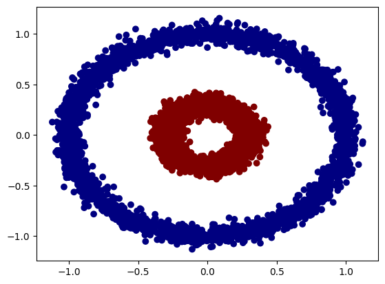
X, y = make_circles(                # load a labelled dataset
    n_samples=5000,
    noise=0.05,
    factor=0.3,
    random_state=42)
lens = PCA(2).fit_transform(X)

plt.scatter(lens[:, 0], lens[:, 1], c=y, cmap='jet')

<matplotlib.collections.PathCollection at 0x7f7a5deda890>

Build Mapper graph

mapper_algo = MapperAlgorithm(
    cover=CubicalCover(
        n_intervals=10,
        overlap_frac=0.3),
    clustering=DBSCAN())

mapper_graph = mapper_algo.fit_transform(X, lens)

Plot Mapper graph with mean

mapper_plot = MapperPlot(
    X, mapper_graph,
    colors=y,                       # color according to categorical values
    cmap='jet',                     # Jet colormap, for classes
    agg=np.nanmean,                 # aggregate on nodes according to mean
    dim=2,
    iterations=60,
    seed=42)

fig_mean = mapper_plot.plot(
    width=600,
    height=600)

fig_mean.show(renderer='notebook_connected', config={'scrollZoom': True})

fig_std = mapper_plot.with_colors(  # reuse the plot with the same positions
    colors=y,
    cmap='viridis',                 # viridis colormap, for ranges
    agg=np.nanstd,                  # aggregate on nodes according to std
).plot(
    width=600,
    height=600)

fig_std.show(renderer='notebook_connected', config={'scrollZoom': True})